Random-Number Generation

Tests for Random Numbers

Two categories:

Testing for uniformity:

Failure to reject the null hypothesis, H₀, means that evidence of
non-uniformity has not been detected.

Testing for independence:

independently
independently

Failure to reject the null hypothesis, H₀, means that evidence of
dependence has not been detected.

Level of significance α, the probability of rejecting H₀ when it
is true:

α = P(reject H₀|H₀ is true)

When to use these tests:

If a well-known simulation languages or random-number
generators is used, it is probably unnecessary to test
If the generator is not explicitly known or documented, e.g.,
spreadsheet programs, symbolic/numerical calculators, tests
should be applied to many sample numbers.

Types of tests:

Theoretical tests: evaluate the choices of m, a, and c without
actually generating any numbers
Empirical tests: applied to actual sequences of numbers
produced. Our emphasis.

Frequency Tests [Tests for RN]

Test of uniformity

Two different methods:

Kolmogorov-Smirnov test
Chi-square test

Kolmogorov-Smirnov Test [Frequency Test]

Compares the continuous cdf, F(x), of the uniform
distribution with the empirical cdf, S_N(x), of the N sample
observations.

We know: F(x) = x, 0 ≤ x ≤1
If the sample from the RN generator is , then the
empirical cdf, S_N(x) is:

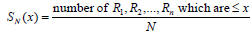
Based on the statistic: D = max| F(x) - S_N(x)|

Sampling distribution of D is known (a function of N, tabulated in
Table A.8.)

A more powerful test, recommended.

Example: Suppose 5 generated numbers are 0.44, 0.81, 0.14,
0.05, 0.93.

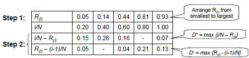
Step 3: Step 4: For α = 0.05, = 0.565 > D Hence, H0 is not rejected.

Chi-square test [Frequency Test]

Chi-square test uses the sample statistic:

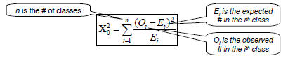
Approximately the chi-square distribution with n-1 degrees of
freedom (where the critical values are tabulated in Table A.6)
For the uniform distribution, E_i, the expected number in the each
class is:

,where N is the total # of observation

Valid only for large samples, e.g. N >= 50

Tests for Autocorrelation [Tests for RN]

Testing the autocorrelation between every m numbers
(m is a.k.a. the lag)

The autocorrelation between numbers:

M is the largest integer such that i +(M +1)m ≤ N

Hypothesis:

   if numbers are independent
, if numbers are dependent

If the values are uncorrelated:

For large values of M, the distribution of the estimator of ,
denoted is approximately normal.

Test statistics is:

Z₀ is distributed normally with mean = 0 and variance = 1

If > 0, the subsequence has positive autocorrelation

High random numbers tend to be followed by high ones, and vice versa.

If < 0, the subsequence has negative autocorrelation

Low random numbers tend to be followed by high ones, and vice versa.

Shortcomings [Test for Autocorrelation]

The test is not very sensitive for small values of M,
particularly when the numbers being tests are on the low
side.

Problem when “fishing” for autocorrelation by performing
numerous tests:

If α = 0.05, there is a probability of 0.05 of rejecting a true
hypothesis.
If 10 independence sequences are examined,

The probability of finding no significant autocorrelation, by
chance alone, is 0.95¹⁰ = 0.60.
Hence, the probability of detecting significant autocorrelation
when it does not exist = 40%